AP Physics C: Mechanics Standards 2013-14

I've finished revising my standards for AP Physics C: Mechanics for next year. The standards that I used last year were a little too grainy, for the most part, for my liking. I prefer having each model as a standard, with the specific content and skills subordinate to that model as indicators. This means that reassessments don't suffer as much from the "cherry picking" of students choosing isolated and unrelated skills to reassess. Because each reassessment is on a whole model, even a student that only had an issue with elastic collisions would still have to reassess on all of the related skills - identifying when CopM applies, deal with other types of collisions, etc. and demonstrating sustained mastery. This also keeps the number of reassessments that I have to make lower, with only 8-12 standards per term.

The standards reflect a hybrid AP/Matter and Interactions approach (I'm using Knight's Physics for Scientists and Engineers for the first time this year, alongside M and I). I weave the two together, including the topics that the AP curriculum covers that M and I doesn't and the larger narrative and inclusion of programming and modern physics of M and I.

The overview:

• Fall Term (the momentum principle)
• Unit 1: motion (constant and non-constant a and forces), drag, oscillations (springs and others, but not pendula), intro to Python
• Unit 2: momentum principle, momentum (conservation and impulse), circular motion (uniform and non-uniform), non-inertial reference frames
• Unit 3: chaos, relativistic momentum, materials (ball and spring model of matter, speed of sound, Young's modulus)
• Winter Term (the energy principle)
• Unit 4: work, power, relating U and F, gravitational and electrical potential energy, universal gravitation and orbits, conservation of E
• Unit 5: quantized energy (spectra), relativistic energy, mass energy
• Unit 6: real and point-particle systems, moment of inertia, conservation of energy with rotation
• Spring Term (the angular momentum principle)
• Unit 7: angular momentum conservation, torque, static equilibrium
• Unit 8: unbalanced torques, angular motion
• Unit 9: statistical mechanics: micro/macrostates, entropy, temperature, specific heat, Boltzmann distributions

Here are PDFs for the standards:

• Fall
• Winter
• Spring

Automatic Email Responses for Google Form Submissions

Since I use a Google form for student reassessment requests (very helpful, BTW), I've often had students forget what standard they registered for or which day or had "but I submitted it!" issues.

This script should solve that. In the form edit window, go to Tools and Script Editor, and add a script to your form.

Here's my script (modify to suit your needs):

function onFormSubmit(e) { 
 // these are the columns in the form:   
  var timestamp = e.values[0];
  var yourName = e.values[1];
  var Section = e.values[2];
  var std = e.values[3];
  var ReDate = e.values[4];

  var toAddress = e.values[5];

  var subject = "Reassessment Confirmation - " + std + " " + ReDate;
  var emailBody = "You requested a reassessment on: " + timestamp +      " for " + std +      ". \n\nThe reassessment will take place on " + ReDate +      ".";

  MailApp.sendEmail(toAddress, "you@yourschool.edu", subject, emailBody);
}

The last thing that you need to give the script permission to send emails. Go To Resources/All Your Triggers -> Run OnFormSubmit Events From Spreadsheet -> OnFormSubmit.

There are optional arguments for the sendEmail method that let you send fancy HTML emails, but this will work OK for me.
Enjoy!

Dragging out Drag

My sequence for drag for the AP class next year:

• Coffee filter investigation primarily about the kinematics of the motion (not working with the forces, except as derived through the motion analysis)
• They draw a predicted position graph, having seen the filter float downward
• Measure with motion detector, check prediction
• Predict velocity graph shape
• Check with motion detector
• Predict acceleration graph shape
• Some questions about interpreting the initial and final slopes of the y and v graphs and the concavity of the y graph's relationship to the acceleration
• Assuming a velocity of this form:, determine the meanings of the constants, a velocity function, the terminal velocity, an acceleration function, and - finally - an expression for the net force (in terms of the velocity)
  
  
• A few weeks later, another coffee filter modeling investigation, centering on using linearization to determine the exponent in the drag force (is it linear or quadratic drag?)
• They'll start from force considerations and determine a way to measure the terminal velocity of their filter
• They'll linearize (either with guesses for the exponent or log/log) to determine the exponent
• They'll use that relationship and the data to calculate the drag coefficient for the filters and compare to some know ones (ie: Wikipedia)

• The next day, start with a terminal velocity exploration:
• Everybody picks an object
• Research and/or estimate necessary quantities
• Determine the terminal velocity of the object
• Sketch position, velocity, and acceleration graphs for your object and a neighbor's object, on the same axes. Make it clear what differences there are and why, and show where the terminal velocity shows up on both the position and velocity graphs
• I'll use the drag graph check Python program below to run through a few of the combinations for them - clear up any remaining issues

• End the day with drag integrals:
• We'll go through separation of variables and see why we don't normally do the integral for quadratic drag. It's a good moment to expose them to the concept of integral tables, which they often seem never to have seen before.
• I'll have them go through free fall and a car rolling to rest with linear drag, so that they have some practice with the calculus. The limits typically trip students up, and these integrals show up on the AP exam at least every other year, so they're good to practice, even if the drag never really is linear

• Maybe at some later point, I'll have them do something with the dashpot setup that I have, but it's fairly close to the second filters lab...

The code:

Relative Velocity and Shaky Cams

I'm working on some of the first few days in AP C next year, and we're doing relative velocity then. I don't really have time to do it in Honors these days, and the AP kids certainly get on top of it very quickly, so I can really put it to bed in about a day with them if I wait, instead of needing a little more time the year before and then taking some time to do some review applications in the second year.

Anyway, here's my progression for that day (95 minutes):

• Frame the need with a video. I made this shaky-cam video of a ball rolling on a table (click through to see video). The motion's certainly odd, with direction changes that seem strange. I only show this one at full speed. Update: here's a link to the video.

• We use Logger Pro to track and model the motion, and the position graphs definitely look weird. Point out to them during the process that they can get a sense for how the speed is changing by looking at the sizes of the blurs. Speed and direction are changing, and (maybe) they won't be able to pick out the underlying motion at this point. 

• Now that we know that there's an issue to be solved and they have discussed the differences between looking at the motion from the camera's POV and the table's POV, I introduce an easier question to tackle, Dan Meyer's escalator/stair video, which they develop a method to solve pretty easily and successfully (though not super-quickly, with the data-taking and wringing of hands about distances and natural units):

Boat In The River — Question from Dan Meyer on Vimeo.

• If we are to apply this model to the first problem to determine what the motion really was, we can add calculated columns in Logger Pro to un-shake the motion and determine what type of motion it really was. Scaling the video (ball diameter is 3.3 cm) lets you calculate initial v and angle, acceleration, etc. as well, if you're into that sort of thing.

I want to seed the concept early and revisit it a few times during the term, so that going to the center-of-mass reference frame for collisions isn't as much of an abstract stretch as it could be.

Variable Mass Half-Atwood

I'm working on my progression of variable-acceleration systems for next year's AP Physics C:Mechanics class. So far, here's the broad outline:

• Constant a systems
• Mostly review; include Atwoods, etc., with new twist of considering the whole system at once, instead of eliminating the tension via algebra. I don't do this with the first-year students because I think that it requires just a little too much intuition and understanding of Newton's laws for where they are
• Variable a: Abstracted 
• Some 'book' problems, involving forces that vary as a function of time, just to incorporate some functions into the net force equations, get used to doing the calculus in that context, etc. Nothing actually new here, since they will be very good at force problems and will have already done time-dependent kinematics work earlier in the term
• Variable a: Half-Atwood
• An experiment involving modeling the flow rate of sand from a bottle and predicting the v(t) function, knowing that. Take data and fit the curve to (hopefully) see agreement. See more below.
• Variable a: Massive Rope
• Atwood machine with a massive rope or a chain of paperclips acting as a half-Atwood on a slick table - either way, set up the differential equation, remark that it's difficult to solve (because of the initial values), maybe look up the sinh function, see that energy's really the way to go when things are function of position.
• Variable a: Drag
• Work on system where force is a function of v; maybe I'll post this one later - it's the second of two coffee filter labs, this one working on modeling the force and linearization, followed by doing those linear drag force integrals that the AP folks love so much. I'm also trying to get something going with a dashpot that I found in the back room, but I'll need some pulleys too, because it's quite small

OK, on to the half-Atwood. It took a couple of days to figure out the experimental setup here, but I think that I have good results, finally. I'll give you the benefits of my frustration :)

First (this isn't super-necessary), I want the kids to model the flow rate of sand as a function of the area of the hole through which it's passing. It's another chance to do some linearization, which was a tool that I really want them to be familiar with by the end of the AP year. They'll think about variables, choose "hole size" probably, which we'll frame as area, then I have some stoppers and such to let the sand go through (don't forget to use no stopper at all, too):

They'll individually test these by hanging the setup from a force probe and fitting a line (it's fairly linear, really). Then they can model the relationship, try a few curves, and I'll suggest linearization. Actually, I'll have to introduce it, because this will be the first time that they see it, I think (I don't use it in the first year because it doesn't work for all kinds of functions and I'd rather them interpret all three coefficients in something like the x(t) function than simplify the situation so that it can be linearized). I got a dependence proportional to the area to the 1.5, though this reference says that it should be 1.25.

Setup:

 Mass as a function of time:

 log-log graph of flow rate and hole area:

This is really only needed so that we can argue that the mass changes linearly in time; I'm even finding the rate via curve-fitting later, so this can be skipped.

I needed a nice long run to get enough data, so I set up some pulleys to extend the run and used a 2.2m Pasco track:

There are some tricks here:

• A recycling basket catches the sand nicely, though dust is an issue
• Put more sand in than you need; it'll give you time to stabilize everything, start the data collection, etc.
• You want a fast flow rate - I used the three-hole cap, but maybe a single larger hole would be even better. I think that no hole might be too fast, but I haven't tried it yet. You don't want the sand to run out during the data run.
• You want a long time, so release the system when the sand is only a couple of second from running out
• Use the Vernier motion detector 2 (green one), because it tracks well all the way up to about 15 or 20 cm from the detector. With the original (blue), I have to be almost half a meter away to get good tracking. 
• I used the Pasco Atwood machine pulley set at the top, a super pulley with the beefier table clamp at the bottom (to stop rotation)

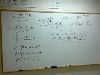
The derivation:

The analysis was done with Logger Pro. The curve at the end of the v graph is only noticeable because the run is long and the acceleration is slow enough to make that happen.

I used the 'Define Function' in the curve analysis, entering the result from the integral, with the flow rate k and the initial mass (called M in the model, but m_0 in my derivation) as parameters. The initial mass was probably around 85 g actually. The flow rate was measured earlier with the three-holed cap as .0176 kg/s, and I get .0135 kg/s here. Between the shape agreement and the reasonable-enough parameter values, I'm happy enough to let the kids do this one in the fall.

I didn't find much with actual experimental application of this system - do you have experience with it? I know that there's some difference in flow rate because of the acceleration, but that's another good reason to keep the acceleration quite small!

Advice to Future Physics Students

This year, I had my students (physics, honors physics, and AP physics) this year write some advice to future students, paying forward their experience: things to do, things not to do, encouragement, etc.

I was very pleased with the types of things that they advised, and I put together a sheet for next year's packets with some highlights. The file's linked here, but I thought that I'd also share the process for making these (with the rotating font sizes, types, and styles) yourself:

• You'll need Python (script below) and LaTeX
• Type the advice into a plain text document (UTF-8 encoding, so that the apostrophes don't get lost in the LaTeX), one nugget per line
• I had it print only lines with * at the end, so that I could save all of the advice, but only use some of it. You can certainly modify the code to fit your needs
• You'll need to make a few path and file mods (it's also calling Preview at the end to display, so if you're not on OSX you'll need to change that too)
• Run and enjoy - let me know if you found it useful!

The script (quick and dirty - surely can be improved. For example, most of the imports don't really need to be there, but I was modifying an old script, and they weren't hurting anyone):