Monday, December 2, 2013

Independent Friction Labs and Another Capstone Project

I have my Honors Physics students prepare small electronic posters for their final lab of the first term, the Independent Friction Lab. In this lab, students have to come up with an experiment, make an informal proposal, execute the experiment, and analyze the results.

The experiment really just needs to have something to do with friction, and I get a wide variety of them. I have them create a single PP or similar slide, sized 24"x18"; they're great to print at Staples. I ask them to email me a draft a day or so before the presentations, and they present the revised projects.
Here are a few of this year's experiments:

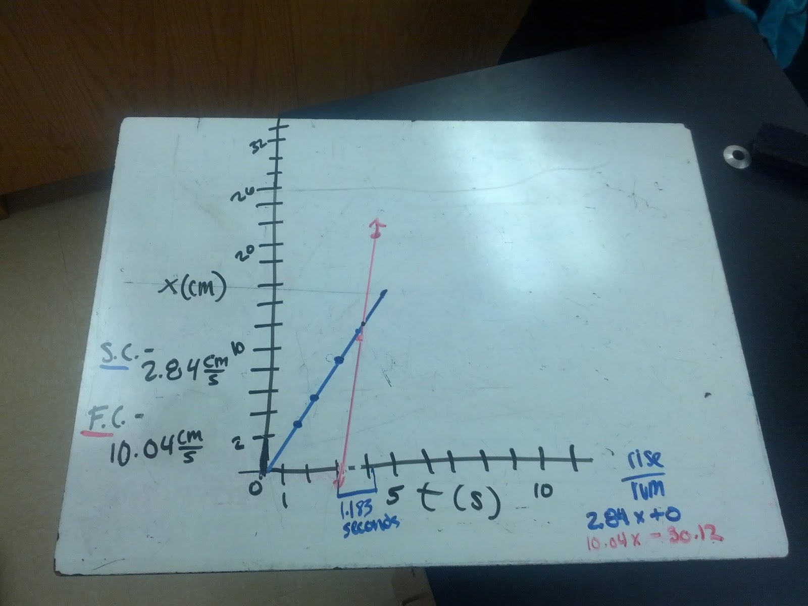
This group used a Pasco friction cart; they let it slide on a cart track, used the velocity graph to determine the coefficient of kinetic friction, and then determined the hanging mass that would pull the friction cart at constant speed (verifying that with another motion detector graph).

This group found the coefficient of static friction between a block and a ramp in a neat way: they used a half-Atwood setup, changing the mass until the block slipped, but performed that experiment at several angles. They then predicted a function for that maximum mass as a function of the block's known mass, the angle, and the unknown friction coefficient. Graphing their data, Logger Pro found the static friction coefficient by regression, providing both a quality value and confirmation of the model that they used to describe the situation.

These students compared the effective coefficients of friction for a ball rolling (without slipping) and the same ball under backspin (backspin persists until it turns around). They're essentially determining the coefficients of rolling and kinetic friction, showing that the kinetic friction coefficient's much larger.

This one seems to come up every year, and it's always fun. They used video analysis to determine the coefficient of kinetic friction between socks and several surfaces. The tricky unseen part is the big possible variation in normal force from foot to foot and moment to moment

A second AP Physics capstone project is also included here; the student was trying to model the interaction between a hockey stick and a puck. It ended up being a very difficult problem, but he gained some valuable ground and ended up with a functional scaled-back model.

Student work:

For my capstone project, I wanted to model the interaction between the blade of a hockey stick and the puck during a shot or pass in ice hockey. Using the ball and spring model of matter interactions, I created a VPython program where a constant force acts on the blade of the stick, but reverses direction at the center (0,0,0) to simulate the slowing down of the stick after reaching the midpoint where the x component of the force on the stick would be at its maximum. The force on the puck, however, does not follow the same constant pattern. Since materials act like springs with miniscule stretches, the force on the puck oscillates during the entire blade-puck interaction time even though the oscillation and resulting compression of the blade would be impossible to see with the naked eye. While this is not a perfect model since the blade remains at a constant angle, 90°, and the force magnitude remains constant in the direction of velocity and only changes direction by 180°, it does illustrate how matter interacts at the atomic scale. During the collision, both the force on the puck and the compression of the blade oscillate, but so slightly with the large spring constant that, looking at the velocity graph, the puck behaves like it would with a constant force and constant acceleration during contact. 


Screenshot at the moment of collision

Graphs of the "spring" compression, force exerted on the puck, and velocity of the puck as functions of time

from __future__ import division
from visual.graph import*
from visual import*

#create objects
h=.025
puck=cylinder(pos=(1,0,0),radius=0.038, height=h, axis=(0,h,0), mass=.17, velocity=vector(0,0,0))


l=.76
R=vector(0,((2l)**2-puck.radius**2)**.5,0)
l=.02
beginpos=vector(puck.pos.x+puck.radius+l/2,puck.height,0)


stick=box(pos=beginpos, length=l, height=.076, width=0.3175, material=materials.wood, velocity=vector(0,0,0), mass=.7,)# axis=norm(R-beginpos)*.076, k=500000)

#R=vector(0,((2l)**2-stick.pos.x**2)**.5,)


scene.autoscale = False

#create forces

Fdirection=vector(-1,0,0)#norm(vector(-stick.axis.y, stick.axis.x,0))

Fmag=200

k= 10000#310575#414172.6


r=puck.pos+vector(puck.radius, puck.height/2,0)-stick.pos

s=stick.length/2-(stick.pos.x-puck.pos.x-puck.radius)  #stick.height/2-(r.mag)*cos(arctan(abs(stick.axis.y/stick.axis.x)))

Fp=vector(k*s*Fdirection)

Fs=Fmag*Fdirection


#graph
gd =gdisplay(x=0, y=0, width=600, height=150, title='Fp vs. t', xtitle='t (s)', ytitle='Fp (N)', foreground=color.black, background=color.white, xmax=.25, xmin=0, ymax=100, ymin=-100)

Fpg=gcurve(color=color.red, gddisplay=gd)


gd2 =gdisplay(x=0, y=0, width=700, height=150, title='compression vs. t', xtitle='t (s)', ytitle='Compression (m)', foreground=color.black, background=color.white, xmax=.25, xmin=0, ymax=.01,ymin=-.005)

sg=gcurve(color=color.green, gdisplay=gd2)

vg = gdisplay(x=0, y=0, width=600, height=150, title='v vs. t', xtitle='t (s)', ytitle='Puck Velocity (m/s)',foreground=color.black, background=color.white, xmax=.25, xmin=0, ymax=0,ymin=-30)
            

vg=gcurve(color=color.blue, display=vg)

print s
#create loop

t=0
dt=.00001

while t<.25:

    rate(10000)

    if s>0 and stick.pos.x>0:
        
        #stick 

        stick.velocity.x=stick.velocity.x+Fs.x/stick.mass*dt

        stick.pos.x=stick.pos.x+stick.velocity.x*dt

   #     R=vector(0,((2*l)**2-stick.pos.x**2)**.5,0)

#        stick.axis=norm(R-stick.pos)*stick.length

        #puck

        puck.velocity.x=puck.velocity.x+Fp.x/puck.mass*dt

        puck.pos.x=puck.pos.x+puck.velocity.x*dt

        #s

        r=puck.pos+vector(puck.radius, puck.height/2,0)-stick.pos

        s=stick.length/2-(stick.pos.x-puck.pos.x-puck.radius)  #stick.height/2-(r.mag)*cos(arctan(abs(stick.axis.y/stick.axis.x)))

        Fdirection=vector(-1,0,0)#norm(vector(-stick.axis.y, stick.axis.x,0))

        Fp=vector(k*s*Fdirection)

        Fs=Fmag*Fdirection-Fp


    elif stick.pos.x>0:
        #stick 

        stick.velocity.x=stick.velocity.x+Fs.x/stick.mass*dt

        stick.pos.x=stick.pos.x+stick.velocity.x*dt

#        R=vector(0,((2*l)**2-stick.pos.x**2)**.5,0)

#        stick.axis=norm(R-stick.pos)*stick.length

        #puck

        puck.velocity.x=puck.velocity.x+Fp.x/puck.mass*dt

        puck.pos.x=puck.pos.x+puck.velocity.x*dt

        #s
        r=puck.pos+vector(puck.radius, puck.height/2,0)-stick.pos

        s=stick.length/2-(stick.pos.x-puck.pos.x-puck.radius)  #stick.height/2-(r.mag)*cos(arctan(abs(stick.axis.y/stick.axis.x)))

        Fdirection=vector(-1,0,0)#norm(vector(-stick.axis.y, stick.axis.x,0))
        Fp=vector(k*s*Fdirection)

        Fs=Fmag*Fdirection

    elif stick.pos.x<0: abs="" arctan="" cos="" fdirection="vector(1,0,0)#norm(vector(-stick.axis.y," fp.x="" fp="vector(k*s*-Fdirection)" fs="Fmag*Fdirection" if="" puck.height="" puck.pos.x="puck.pos.x+puck.velocity.x*dt" puck.velocity.x="puck.velocity.x+Fp.x/puck.mass*dt" puck="" r.mag="" r="puck.pos+vector(puck.radius," s="stick.length/2-(stick.pos.x-puck.pos.x-puck.radius)" stick.axis.x="" stick.axis.y="" stick.axis="norm(R-stick.pos)*stick.length" stick.height="" stick.pos.x="stick.pos.x+stick.velocity.x*dt" stick.pos="" stick.velocity.x="stick.velocity.x+Fs.x/stick.mass*dt">0:
            Fp.x=0


        if stick.velocity.x>0:
            stick.velocity.x=0

        if s<0: abs="" arctan="" cos="" else:="" fp.x="" fpg.plot="" pos="(t," pre="" print="" puck.pos.x="puck.pos.x+puck.velocity.x*dt" puck.velocity.x="" puck.velocity="" r.mag="" s="" sg.plot="" stick.axis.x="" stick.axis.y="" stick.height="" stick.velocity.x="" t="t+dt" vg.plot="">

Wednesday, November 13, 2013

Capstones! Gravitational Slingshot edition

My AP class does capstone projects at the end of each term. It's a short independent project, having to do with anything from the term, which they execute and present in such a way that we can post them here.

Here's the first of the crop of this fall's capstones: a VPython project simulating a gravity assist.

Student work:
The goal of my Capstone project was to create a program in VPython which simulates the gravitational slingshot used by satellites such as Voyager I or Cassini.  This method, officially called “gravity assist”, is used by space programs such as NASA to send probes to distant targets without draining resources since it uses the natural gravitational forces as ways to propel the probes into space.

In the program, I send a 15,000 kg probe into orbit around the Earth while also having the Moon orbit the Earth.  By adjusting the initial velocity of the probe, the probe would be able to pass by the moon and use the Moon’s gravitational force to “slingshot” it off to a “target” asteroid away from the Earth.  Finally, I graphed the speed of the probe during its journey and compared it to the velocity graph of Cassini.  The small boost in the graphs shows the moment the probe uses the gravitational slingshot, similar to the Cassini graph when it orbits around Venus.

Images:
Cassini's speed graph (wikipedia)

The program, after probe has made it to the target

v graph from the program, showing the boost

Cassini Graph citation:

 "Cassini's Speed Related to the Sun." Chart. Wikipedia. Wikimedia, n.d. Web. 12 Nov. 2013. .

Code (syntax highlighting finally works!):
    from __future__ import division
    from visual.graph import*
    from visual import*

    #Richie Lou
    #Gravitational Slingshot - CAPSTONE

    #OBJECTIVE: to use a gravitational force to send a space shuttle from Earth's orbit
    #to a target asteroid by using the moon as a gravitational slingshot

    #Create Shuttle
    Shuttle=box(pos=(6.4e7,0,0), length=72.8, width=108.5, height=20, color=color.red, make_trail=True)
    Shuttle.m=15000 #kg
    Shuttle.v=vector(0,-3350,0) #m/s

    #Create Earth
    Earth=sphere(pos=vector(0,0,0), radius=6.4e6, material=materials.BlueMarble)
    Earth.m=6e24 #kg

    #Create Moon
    Moon=sphere(pos=vector(0,4e8,0), radius=1.75e6, color=color.white, make_trail=True)
    Moon.m=7e22 #kg
    Moon.v=vector(1050,0,0) #m/s

    #Create Target Asteroid
    Target=sphere(pos=vector(-1.40837e9, 1.42004e9, 0), radius=7e6, color=color.green)

    #Create Initial Conditions
    G=6.67e-11 #N*(m/kg)^2 #Gravitational Constant

    R=Shuttle.pos-Moon.pos #m
    r=Shuttle.pos-Earth.pos #m

    M=Moon.pos-Earth.pos #m

    F=Shuttle.pos-Target.pos #m

    FnetShuttle=-(G*Earth.m*Shuttle.m*r)/(mag(r)**3)-(G*Moon.m*Shuttle.m*R/(mag(R)**3)) #N
    FnetMoon=-(G*Earth.m*Moon.m*M)/(mag(M)**3)+(G*Moon.m*Shuttle.m*R/(mag(R)**3)) #N

    deltat=50 #s
    t=0 #s

    #Graph Velocity
    gdisplay(x=0, y=0, width=600, height=150, title="velocity vs. time", xtitle="t", ytitle="velocity (m/s)", foreground=color.black, background=color.white)
    g=gcurve(color.red)

    #Animate Orbit
    while mag(R) > 1.75e6 and mag(r) > 6.4e6 and mag(F) > 7e6:
        Shuttle.pos=Shuttle.pos+Shuttle.v*deltat #m #position update
        Shuttle.v=Shuttle.v+(FnetShuttle/Shuttle.m)*deltat #m/s #velocity update

        Moon.pos=Moon.pos+Moon.v*deltat #m #position update
        Moon.v=Moon.v+(FnetMoon/Moon.m)*deltat #m/s #velocity update

        R=Shuttle.pos-Moon.pos #m
        r=Shuttle.pos-Earth.pos #m

        M=Moon.pos-Earth.pos #m

        F=Shuttle.pos-Target.pos #m

        FnetShuttle=-(G*Earth.m*Shuttle.m*r)/(mag(r)**3)-(G*Moon.m*Shuttle.m*R/(mag(R)**3)) #N #Force update
        FnetMoon=-(G*Earth.m*Moon.m*M)/(mag(M)**3)+(G*Moon.m*Shuttle.m*R/(mag(R)**3)) #N #Force update

        t=t+deltat #s #time update

        rate(1e100)

        g.plot(pos=(t,mag(Shuttle.v)))

    print t/8.64e4, "days"
    print mag(Shuttle.v), "m/s"


Thursday, September 26, 2013

Drag Graphs and Terminal Velocity

This summer, I posted my progression on drag here. One of the new elements was a pair activity where students each calculate the terminal speed of some random object that they come up with and draw (on the same set of axes) the position, velocity, and acceleration curves for the two objects. I then put the values into a VPython script and we check.

We did that today, for the first time, and it went pretty well. The students picked an iPad vs. a calculator and a big (1m on a side) metal box vs. a 747 (nose first). Here's what they got:
iPad (red), calculator (blue)

Neat that the heavier iPad had a lower terminal speed - it's much bigger!

747 (red), box (blue)

That 747 didn't even come close to getting to its terminal speed from 400 meters: how about from 10,000 meters?
747(red), box (blue)

Not much better there. It took nearly 300 km of fall to get there - very heavy, very low drag coefficient.

It was a bit unwieldy entering the values during class, so I think that I might do a Google form/Googlecl/VPython solution to pull those values in from the cloud next year.

Monday, September 16, 2013

A Two-pulley Practicum

In the AP C: Mechanics course, we're working through some extensions to old models - non-constant acceleration as a more general application of CAPM principles, UFPM with non-constant forces, etc.

Even with constant acceleration and constant forces, there are some more subtle, but very powerful, techniques that we can't do the first time around. The first is the "look at the whole system" approach to force analysis. Instead of analyzing the half-Atwood machine, for example, as a hanging mass and a cart, and eliminating the tension algebraically, we decide that the net force accelerating the system is mg and the total mass of the system is m+M, and it's super easy to get the system's acceleration. I know that some folks do this in the first year, but I like having them draw those two FBDs and really puzzle out how the force sizes relate to each other, and I think that this is just a little too black-box (especially with the change in direction of the motion in the middle) for the first year. It's also really good algebra practice.

We'll do that today, but we'll also take a look at this situation:
This can be really tricky to analyze as either a separate or a combined system, but we can make an observation about the rope that's really helpful. When the cart moves a distance d to the right, the rope's downward motion is complicated by the presence of the pulley, but a little careful diagramming can show that half of that d will end up as a longer right-hand vertical rope, and half will end up as a longer left-hand vertical rope, so that the hanging mass m will only drop d/2. Using that, the acceleration of the hanging mass must be half of the acceleration of the cart, which allows us to really easily solve for the unknown acceleration.


This worked out very well as a practicum for me, using Pasco track, carts, and superpulleys (with 100g clamped into the jaws of the hanging one. The time's long enough (with a cart run of about a meter) to be timed pretty well with a stopwatch.
I think that this does a great job of emphasizing the importance of thinking during the problem-solving process and of adding a new twist to what students might think is a "completed" topic.


Friday, September 13, 2013

Follow-up to the Buggy Lab

In a post yesterday, I shared a new piece of my (WCYDWT) buggy lab: having students mark explicitly on the graph which interval denotes their "answer," and having the other groups interpret the graph to determine what the situation and question were.

I had really only done this with one of two sections of Physics, and I have now had both of those sections a second time after that lab. The results for one task seemed pretty clear. I used Matt Greenwolfe's suggestion here to wrap that up by asking them to draw a specific position vs. time graph for all six robots. I actually asked for two graphs: first, for the six robots, if each was programmed to run for 20 seconds and stop (that's how they were actually programmed on the first day). Second, for the six robots, if each was programmed to run for one meter and stop.

The first class had some of the same issues that Matt described: confusing the time and distance intervals, ascribing meaning to the length of the line, etc. After some discussion, they figured it out and went on. The second class had a much higher proportion of correct graphs from the beginning on both questions. It was a large departure from previous classes' performance as well, so it seems to have had a positive effect.

One of the graphs from the second question is below. The others have been erased, but several of them drew dotted lines horizontally or vertically first, then drew their graphs, which is a great sign.


Wednesday, September 11, 2013

Standards for the Year

We had a great discussion on standards-based grading at the Global Physics Department tonight. Here are my standards for the year for each course, in response to a request from that conversation.

AP Physics:

  • Term 1 (Momentum Principle)
  • Term 2 (Energy Principle)
  • Term 3 (Angular Momentum Principle)
Honors Physics:
  • Term 1 (Motion, Forces)
  • Term 2 (UCM, Gravitation, momentum)
  • Term 3 (Energy, Oscillations, Static Electricity, DC Circuits)
Physics:
  • Term 1 (Motion, Forces)
  • Term 2 (Oscillations, Waves)
  • Term 3 (Sound, Phases/Eclipses/Shadows, Geometric Optics)

A New Twist on the Buggy Lab

I usually do the CVPM buggy lab as a WCYWDT? (What Can You Do With This?) challenge. Here's what that looks like:

  • Each group gets a slow and a fast cart (this year, I'm using the Scribbler 2 robots, along with Matt Greenwolfe's software)
  • Each group has to come up with a unique question - they put the carts into a situation and then make some prediction. Common ones include: "If they start a meter apart, where/when will they collide?" and "How much of a head start (time or distance) does the slow one need in order for the race to be a tie?"
  • Groups take data, using only one cart at a time (no testing before the big reveal!)
  • Groups create position vs. time graphs to answer their questions
  • Along the way, I ask some questions to be sure that they're framing speed correctly (m/s vs. s/m), that they're really representing their situation with the graph (if they don't start at the same place, then they shouldn't on the graph, either), etc.
  • They test their predictions, in front of everyone. These always go well, and I think that the inherent slowness of the Scribblers makes them more dramatic and easier to discern whether the test worked or not.
Here's the new part:
  • As they're finishing up their whiteboards, I have them bracket the answer to the question on their graph - if they're predicting a distance, then they need to show where that distance interval is located on the graph. If it's a time interval, then they need to bracket that, etc.
  • Students do not write their questions on the boards
  • The "presentation": students show their WBs, saying nothing. It's the rest of the class's job to figure out exactly what their situation was and what they were trying to find.
Here's why:
  • Some students have trouble differentiating between a fast car and a slow one and between a race and a head-on collision at this early stage. Having had to go through that process when they drew their graphs, they now get a few more chances to practice those skills immediately after that first experience.
  • Lots of students have difficulty locating different quantities on their graphs. In CVPM, it's not nearly as big a deal, but lots can go off of the rails when trying to find delta v or the final velocity or the displacement, etc. when we get to CAPM, so this is working on those skills early and explicitly.
  • It keeps the viewers actively engaged, much like the mistake game or other similar strategies.
Here are a few examples from today. I really like the fourth on, because the time interval that they were looking for was not starting at zero, but instead from when the second cart started. That's the sort of thing that often trips students up, even if they've drawn a correct graph to begin with.


Friday, August 30, 2013

Reasonable Numbers, Unreasonable Nutrition

I just went to a McDonald's to eat and use the wi-fi to get some work done. Here's how it went down:

  • Ordered 20 pc meal (stop with your judging eyes) 
  • Cashier kid heard 10 pc. I didn't notice until after I had paid. 
  • He called over manager. She decided to see what the price of the 20 pc meal was ($7.50), look at the receipt ($6.19), and charge the difference. 
  • She asked the kid what the difference was. He was pretty satisfied with his answer of $1.20. She found an item for $1.15 and charged me. 
  • Everyone involved was very nice and helpful, and works too hard for too little money.
There are a lot of failure modes for mental arithmetic, but there are some simple checks that you should go through. Here, anything that doesn't end with 1 is impossible. It's easy to come to $1.41 or maybe $1.21, but $1.20 shouldn't pass the smell test. 

We've been doing some curriculum work at school, and the math and science departments across all four divisions are convinced that this sort of answer-checking is something that kids have to have. They're right. It's a habit of mind for a scientist or mathematician, and it's something that we have to spend time with our kids on if we want them to learn it. 

$1.30 as an approximate answer's pretty good, and that's something else that we should work with kids on - coming to first approximations before solving a problem, so that we have some idea about what we're supposed to get, not falling prey to the "writing down whatever the calculator spits out" syndrome. These approximations can be about rounding numbers or about using a first-order Taylor series or squaring off a curve or whatever, but this is a skill that's even less frequently explicitly taught in schools than checking answers for reasonableness. Dan Meyer's "Give me a number that's too high, give me a number that's too low, give me a guess" is a great way to start.

There's certainly a lot of content to get through, but these mathematical practices are arguably at least as important, not least because they'll often survive after the content is forgotten. Don't we want to live in a world where people have these tools (even non-academic folk)? If the answer's yes, then put your class time and assessment questions where your mouth is this year - make time for work on reasonableness-checking and approximation.

Saturday, August 17, 2013

Whiteboard Loudly

I came across "University Buys Bulletproof Whiteboards" today. It's about a move by UM-Eastern Shore to buy 200 18"x20" bulletproof whiteboards - at what seems like a cost of $300 a piece. The idea is that students and teachers can use these as shields in the event of a school shooting. Those logistics aside, two things:

1. This is a far cry from the $2 Interactive Whiteboard! Portable whiteboards are cheap and can instantly transform a classroom into a place of doing, rather than a place of hearing. While it's great that some of these whiteboards are going into UMES, I hope that they're also being used to change the environment of the classroom, rather than sitting next to desks waiting for bad news. For the price, they could buy/make a $2 whiteboard for every student at the school! The cost/benefit analysis here isn't really my point, but if these are worth $60,000, maybe it's also worth it to spend $5000 to outfit every room in the school with a set of student whiteboards, and worth the cost to train teachers to use them effectively to increase student engagement and learning.

2. I generally try to stay away from the bottom half of the internet, but the comments in the CNN article speak volumes. Almost everybody there cannot conceive of whiteboards that are not the exclusive domain of the teacher. (some disturbing images ahead, and, as usual, even more offensive stuff in other comments on the article, so follow those at your own risk)
  • "Sure is a publicity stun[t]. Dumb one at that because it's pretty obvious that a shooter can figure out how to walk behind a white board."
  • "How does a bullet-proof white board, which is mounted against a wall, protect anyone from bullets, which would be fired from somewhere inside the same room?"
  • "The point derpmage is making is that all these whiteboards are mounted (i.e. screwed into the walls) typically in these classrooms. So, if something started, what is a teacher supposed to do? Are they supposed to somehow rip a bulletproof Kevlar Reinforced whiteboard off the wall somehow in order to use it to protect themselves and others? Not going to happen. A waste of taxpayer dollars."
  • "There's a hook for easy hanging. Did you honestly think that you were the only one smart enough to realize that having it bolted to the wall would be problematic? It may be a waste, but they did have the foresight to consider the access issue."
  • "Many whiteboards are used as standalones next to the blackboard... not hung on walls..."
  • "Most schools got away from blackboards and use large whiteboards attached to the walls and use markers. This is really too small for classrooms. It wouldn't hold much information. Besides, the teacher may be safe but not the students. One University building has more then 200 rooms."
  • "You take it off the wall and use it as a shield."
  • "Is the professor supposed to hold the whiteboard -all the time- in preparation for the moment a gunman comes charging through the door? Otherwise they'll be dead before they get to it."
  • "Also, I reckon these whiteboards may be more handy for a crazy gunman than the professor trying to hide behind it. Simply take out professor and ... BINGO, the gunman now has a shield against law enforcement to hold off their position! Super dumb in my opinion."
Even folks that notice the small sizes of the boards go through contortions to imagine them on the wall, in the professor's hand, etc. I haven't seen a single comment understand the idea that the whiteboards are for the students. If you're whiteboarding, don't keep it a secret! It's pretty infectious, so let some teachers see students working actively with whiteboards, figuring things out, collaborating, being skeptical... ; it got me hooked!

A few links about whiteboarding:

Wednesday, July 24, 2013

LaTeX Code for Standards

If you're interested in displaying coarser standards with core skills and proficiency indicators (or whatever you want to call them) in nice LaTeX boxes, here's some code for you!

There are two main templates that I work with - one with a subtitle for the standard and one without. The centering on the vertical text doesn't (in my experience) work, so I just have to play with the size of the parbox to make that work, but everything else renders pretty easily.

Edit: Thanks to Aaron Titus for pointing out two necessary inclusions:
\usepackage{multirow}
\usepackage{graphicx}

No subtitle:


{\footnotesize \begin{tabular}{| p{.7 cm} | p{1.7 cm} | p{13 cm} | }
\hline
\multirow{8}{*}
 {\rotatebox[origin=c]{90}{\parbox{22 mm}{{\large{\bf Friction }}}}}  
&Core Skills & Identify situations in which friction forces are present and understand the microscopic model of friction forces\\ \cline{3-3}
& & Differentiate between static and kinetic friction \\ \cline{2-3}
& \multirow{2}{*}{\parbox{1.7cm}{Proficiency Indicators}} & Determine the direction of the friction force \\ \cline{3-3}
& & Use an appropriate expression for the magnitude of the friction force \\ \cline{3-3}
& & Understand the relationships among normal force, friction force and friction coefficients \\ \cline{3-3}
& & Solve problems using friction \\ \cline{2-3}
& \multirow{1}{*}{\parbox{1.7cm}{Adv. Ind.}} & Solve complex friction problems, including banked curves (not at design speed) \\ \cline{2-3}
\hline
\end{tabular} }
\vspace{2 mm}

Subtitle:
{\footnotesize \begin{tabular}{| p{.15 cm}  p{.15 cm} | p{1.7 cm} | p{13 cm} | }
\hline
\multirow{8}{*}
{\rotatebox[origin=c]{90}{\parbox{32 mm}{{\large{\bf UFPM }}}}}  
&\multirow{8}{*}
{\rotatebox[origin=c]{90}{{\parbox{50 mm}{\scriptsize \centering Unbalanced Force Particle Model}}}} &Core Skills & Recognize when the forces on an object or system are not balanced from observation, graphs, equations, or descriptions of the motion  \\ \cline{4-4}
& & & Identify the presence and directions of normal, tension, and weight forces  \\ \cline{4-4}
& & & Draw a force diagram (FBD) accurately showing directions and types of forces acting on an object or system  \\ \cline{4-4}
& & & Write net force equations describing an object or system; they should indicate that the forces are not balanced in the appropriate dimension(s)  \\ \cline{3-4}
& & \multirow{2}{*}{\parbox{1.7cm}{Proficiency Indicators}} & Draw FBD correctly indicating that forces are not balanced; recognize same \\ \cline{4-4}
& & & Choose and consistently apply workable direction(s) of positive \\ \cline{4-4}
& & & Correctly apply Newton's 3rd law \\ \cline{4-4}
& & & Choose appropriate axes for force analysis \\ \cline{4-4}
& & & Solve problems using net force equations and/or FBD \\ \cline{3-4} 
 \hline
\end{tabular} }
\vspace{2 mm}

Wednesday, July 17, 2013

LaTeX Python Scripts

Here are the supporting materials from my final talk at AAPT's Summer Meeting 2013 in Portland, on LaTeX and Python in assessment creation.

There are two Python scripts and some LaTeX examples in the package. The scripts are:

  • Assessment Maker Lite: takes problems from the problem database (well, really a folder of individual problem LaTeX files) and assembles a properly numbered and pretty assessment PDF
  • Problemdb Lite: manages the problem database: it counts the problems, identifies the tags on each, and renders a PDF based on search criteria ("Vectors Drag" would search for problems containing both tags and "Vectors OR Drag" would get vector problems and drag problems) or gives a PDF of the whole set. Vertical space is removed, so the set will be compressed and will fit in a smaller number of pages, but it may cause awkward display at times.
There are some auxiliary documents, including a LaTeX example document and an Excel sheet to store assessment names and problem numbers for future reference (and easier entry into the Assessment Maker). 

You'll have to set some paths if you move things around, and definitely to reflect the location of your LaTeX engine and PDF viewer. There are comments in the code showing you where you might need to do that.

Any Python install should be fine: I'm using Python 2.7, if you're curious. You'll need a LaTeX install and the only custom style package needed is floatflt (available at CTAN and by Googling).

These can be expanded a great deal, including adding a GUI (I use Tkinter), polling Google docs (using GoogleCL) to create customized reassessments based on student signups, etc. These require more dependencies and directory-setting, so I didn't include them in the Lite versions.

I'm not a software engineer, so there's surely improvement to be made, features to be added, and errors to be checked (it'll just crash out if there's a compile issue, for example), but it should be fine for workaday use - it is for me! :)

Tuesday, July 16, 2013

Stick Figure Maker 1.0

Here's a VPython script that lets you click and drag to create stick figures in any position, so that you can take a screenshot and use them in test questions, etc. It's quick and dirty, but it should work for you, if you have VPython installed.
  • Drag any of the red handles to reposition - the head's not independently movable yet
  • Position the floor, if you need to
  • Click the toggle switch to hide the handles
  • Screenshot
  • Done!
There's a short YouTube video of the process in action here.

Some examples:
Walking
Running
Ninja Attack!
I borrowed the kernel of the drag-and-drop code from Sherwood/Chabay. Let me know if you find it useful!

The source:

Monday, July 15, 2013

SBG Resources

I'm posting some resources from the SBG panel from today. Thanks to everyone that came! Here are some of the resources that we discussed:

Sunday, July 14, 2013

SBG: Philosophy and Logistics

Teaching is always the best way to learn. Yesterday, Andy (SuperFly) Rundquist and I gave a workshop on standards-based grading at the AAPT summer national meeting in Portland. While preparing the workshop, I did several things. Watching all of Portlandia was valuable, but preparing the agenda and having conversations in the workshop were terrific.

Many of these teachers were on the cusp of their first year of SBG implementation, and itching for advice. One of the things that folks are always interested in is the logistics - grading scaling, calculating overall grades, mechanisms for reassessment, etc. The more important part, though, is the philosophy, and everything else is just implementation. If you're not sure what your purposes for assessment are, how that relates to feedback and what the students do next, then the potential benefits will be lost. This is an interesting contrast to traditional grading - because everyone's familiar with traditional grading, you don't actually need to consider why you're doing it, what you want out of it, exactly what the expectations are for the students, etc. That doesn't mean that any particular teacher doesn't, but think about it - do you really need to have a consistent philosophy of assessment to conduct your class and assessments that way? You really don't!

There are as many implementations of SBG as there are teachers, but there are, as I see it, two non-negotiable tenets of SBG:
  1. To the best of your understanding, student understanding and the grade should be interchangeable, equivalent, homeomorphic, or whatever you want to call it.
  2. Understanding changes over time (therefore... so should grades, by application of #1)
A corollary of #1 is that the grades have to be related to the content, rather than the assignments. That's where the standards-based part comes in. How you accomplish these, by grainy or coarse standards, student-initiated or teacher-initiated reassessments, with binary or other rubrics, etc. is highly dependent on your students (age, preparation, numbers), your school (time, culture, schedule), and you (personality, experience, class rapport). As long as you keep #1 and #2 in mind, communicate them to the students often, and everyone's clear that the students and teacher are a team working towards understanding, the implementation details aren't the main thing.

Basically, that's how you survive your first year of SBG. With that under your belt, start worrying about reducing paperwork, streamlining reassessment sign-up and administration, making reporting better, and all of that.

One big discussion that we had involved the inclusion of time as a variable in the grading. This is the default in traditional grading - there's not much reward for learning material after the test, so two students that both learn all of the material and score the same on the final could, because of the speed at which they learned it, get vastly different overall grades. The philosophy of SBG definitely tries to remove time as a variable, and I think that the improvement of grades to reflect improved understanding and the lowering of grades to reflect eroded understanding puts a very clear message out that enduring understanding is all that I care about, not how fast you learn or whether you can cram.

There was a little bit of pushback on that, and a good discussion followed. One idea thrown out was about employers - don't they want to know which person can learn the skill in a day instead of three? Probably they do, but I don't think that the traditional system actually communicates that clearly. Before I get to that, I don't think that it's appropriate to make that sort of thing an issue for novices; we're talking about kids in their first or second class here, not grad students ready to go into the workforce as physicists. 

The more important thing for me is the collateral damage that an attempt to include speed of acquisition by way of not allowing grades to change over time. The argument seems like it's about differentiating between these two kids:
...but in reality, it ends up being these two kids:
Without the incentive structure, support, and learning from assessments (when they're not final, they're easier to really take as indicators for improvement, rather than scarlet "D"s to be ashamed of and thrown away), a good number of those students simply fall of the the back of the pack, having a shaky foundation that they can't build upon. What I'm saying is that, with SBG, the
blue line" kid from the second graph can become the "blue line" kid from the first graph!

I've seen some criticism from others than SBG can allow higher grades than traditional grading. When applied correctly, that's a feature, not a bug.

My grade distribution is about the same as it was before, but each grade represents a higher level of understanding than before. When there's a mechanism to improve, the bar can be higher!

Interestingly, we heard from some local teachers that the state of Oregon is implementing SBG across the board in the near future. That seemed to have driven some of the high attendance in our workshop. I did a little searching, but couldn't find the details on the plan, so corrections/additions/clarifications are welcome in the comments. I'm certainly all for SBG, but it's really dangerous to make big top-down changes to these things. There must be a lot of teacher education and buy-in to make it work, or it'll be another passed ed fad, which would be a tragedy. Philosophy first, logistics second.

OK, tonight a little sushi to talk over the panel discussion on SBG that Aaron Titus, Stephen Collins, SuperFly, and I are leading tomorrow (8-10 in Broadway I/II) and then a day checking out Eugenia Etkina's new text at noon (Pavilion West) and the Demo/Lab (Galleria II) and Modeling instruction (Ballroom II/III) sessions from 4-6.

Sunday, June 30, 2013

AP Physics C: Mechanics Standards 2013-14

I've finished revising my standards for AP Physics C: Mechanics for next year. The standards that I used last year were a little too grainy, for the most part, for my liking. I prefer having each model as a standard, with the specific content and skills subordinate to that model as indicators. This means that reassessments don't suffer as much from the "cherry picking" of students choosing isolated and unrelated skills to reassess. Because each reassessment is on a whole model, even a student that only had an issue with elastic collisions would still have to reassess on all of the related skills - identifying when CopM applies, deal with other types of collisions, etc. and demonstrating sustained mastery. This also keeps the number of reassessments that I have to make lower, with only 8-12 standards per term.

The standards reflect a hybrid AP/Matter and Interactions approach (I'm using Knight's Physics for Scientists and Engineers for the first time this year, alongside M and I). I weave the two together, including the topics that the AP curriculum covers that M and I doesn't and the larger narrative and inclusion of programming and modern physics of M and I.

The overview:
  • Fall Term (the momentum principle)
    • Unit 1: motion (constant and non-constant a and forces), drag, oscillations (springs and others, but not pendula), intro to Python
    • Unit 2: momentum principle, momentum (conservation and impulse), circular motion (uniform and non-uniform), non-inertial reference frames
    • Unit 3: chaos, relativistic momentum, materials (ball and spring model of matter, speed of sound, Young's modulus)
  • Winter Term (the energy principle)
    • Unit 4: work, power, relating U and F, gravitational and electrical potential energy, universal gravitation and orbits, conservation of E
    • Unit 5: quantized energy (spectra), relativistic energy, mass energy
    • Unit 6: real and point-particle systems, moment of inertia, conservation of energy with rotation
  • Spring Term (the angular momentum principle)
    • Unit 7: angular momentum conservation, torque, static equilibrium
    • Unit 8: unbalanced torques, angular motion
    • Unit 9: statistical mechanics: micro/macrostates, entropy, temperature, specific heat, Boltzmann distributions
Here are PDFs for the standards:

Thursday, June 27, 2013

Automatic Email Responses for Google Form Submissions

Since I use a Google form for student reassessment requests (very helpful, BTW), I've often had students forget what standard they registered for or which day or had "but I submitted it!" issues.

This script should solve that. In the form edit window, go to Tools and Script Editor, and add a script to your form.

Here's my script (modify to suit your needs):

function onFormSubmit(e) { 
 // these are the columns in the form:   
  var timestamp = e.values[0];
  var yourName = e.values[1];
  var Section = e.values[2];
  var std = e.values[3];
  var ReDate = e.values[4];

  var toAddress = e.values[5];

  var subject = "Reassessment Confirmation - " + std + " " + ReDate;

  var emailBody = "You requested a reassessment on: " + timestamp +      " for " + std +      ". \n\nThe reassessment will take place on " + ReDate +      ".";

  MailApp.sendEmail(toAddress, "you@yourschool.edu", subject, emailBody);
}

The last thing that you need to give the script permission to send emails. Go To Resources/All Your Triggers -> Run OnFormSubmit Events From Spreadsheet -> OnFormSubmit.

There are optional arguments for the sendEmail method that let you send fancy HTML emails, but this will work OK for me.
Enjoy!

Tuesday, June 25, 2013

Dragging out Drag

My sequence for drag for the AP class next year:

  • Coffee filter investigation primarily about the kinematics of the motion (not working with the forces, except as derived through the motion analysis)
    • They draw a predicted position graph, having seen the filter float downward
    • Measure with motion detector, check prediction
    • Predict velocity graph shape
    • Check with motion detector
    • Predict acceleration graph shape
    • Some questions about interpreting the initial and final slopes of the y and v graphs and the concavity of the y graph's relationship to the acceleration
    • Assuming a velocity of this form:, determine the meanings of the constants, a velocity function, the terminal velocity, an acceleration function, and - finally - an expression for the net force (in terms of the velocity)

  • A few weeks later, another coffee filter modeling investigation, centering on using linearization to determine the exponent in the drag force (is it linear or quadratic drag?)
    • They'll start from force considerations and determine a way to measure the terminal velocity of their filter
    • They'll linearize (either with guesses for the exponent or log/log) to determine the exponent
    • They'll use that relationship and the data to calculate the drag coefficient for the filters and compare to some know ones (ie: Wikipedia)
  • The next day, start with a terminal velocity exploration:
    • Everybody picks an object
    • Research and/or estimate necessary quantities
    • Determine the terminal velocity of the object
    • Sketch position, velocity, and acceleration graphs for your object and a neighbor's object, on the same axes. Make it clear what differences there are and why, and show where the terminal velocity shows up on both the position and velocity graphs
    • I'll use the drag graph check Python program below to run through a few of the combinations for them - clear up any remaining issues

  • End the day with drag integrals:
    • We'll go through separation of variables and see why we don't normally do the integral for quadratic drag. It's a good moment to expose them to the concept of integral tables, which they often seem never to have seen before.
    • I'll have them go through free fall and a car rolling to rest with linear drag, so that they have some practice with the calculus. The limits typically trip students up, and these integrals show up on the AP exam at least every other year, so they're good to practice, even if the drag never really is linear
  • Maybe at some later point, I'll have them do something with the dashpot setup that I have, but it's fairly close to the second filters lab...
The code:

Friday, June 21, 2013

Relative Velocity and Shaky Cams

I'm working on some of the first few days in AP C next year, and we're doing relative velocity then. I don't really have time to do it in Honors these days, and the AP kids certainly get on top of it very quickly, so I can really put it to bed in about a day with them if I wait, instead of needing a little more time the year before and then taking some time to do some review applications in the second year.

Anyway, here's my progression for that day (95 minutes):
  • Frame the need with a video. I made this shaky-cam video of a ball rolling on a table (click through to see video). The motion's certainly odd, with direction changes that seem strange. I only show this one at full speed. Update: here's a link to the video.
  • We use Logger Pro to track and model the motion, and the position graphs definitely look weird. Point out to them during the process that they can get a sense for how the speed is changing by looking at the sizes of the blurs. Speed and direction are changing, and (maybe) they won't be able to pick out the underlying motion at this point. 
  • Now that we know that there's an issue to be solved and they have discussed the differences between looking at the motion from the camera's POV and the table's POV, I introduce an easier question to tackle, Dan Meyer's escalator/stair video, which they develop a method to solve pretty easily and successfully (though not super-quickly, with the data-taking and wringing of hands about distances and natural units):
  • If we are to apply this model to the first problem to determine what the motion really was, we can add calculated columns in Logger Pro to un-shake the motion and determine what type of motion it really was. Scaling the video (ball diameter is 3.3 cm) lets you calculate initial v and angle, acceleration, etc. as well, if you're into that sort of thing.
I want to seed the concept early and revisit it a few times during the term, so that going to the center-of-mass reference frame for collisions isn't as much of an abstract stretch as it could be.

Thursday, June 20, 2013

Variable Mass Half-Atwood

I'm working on my progression of variable-acceleration systems for next year's AP Physics C:Mechanics class. So far, here's the broad outline:
  • Constant a systems
    • Mostly review; include Atwoods, etc., with new twist of considering the whole system at once, instead of eliminating the tension via algebra. I don't do this with the first-year students because I think that it requires just a little too much intuition and understanding of Newton's laws for where they are
  • Variable a: Abstracted 
    • Some 'book' problems, involving forces that vary as a function of time, just to incorporate some functions into the net force equations, get used to doing the calculus in that context, etc. Nothing actually new here, since they will be very good at force problems and will have already done time-dependent kinematics work earlier in the term
  • Variable a: Half-Atwood
    • An experiment involving modeling the flow rate of sand from a bottle and predicting the v(t) function, knowing that. Take data and fit the curve to (hopefully) see agreement. See more below.
  • Variable a: Massive Rope
    • Atwood machine with a massive rope or a chain of paperclips acting as a half-Atwood on a slick table - either way, set up the differential equation, remark that it's difficult to solve (because of the initial values), maybe look up the sinh function, see that energy's really the way to go when things are function of position.
  • Variable a: Drag
    • Work on system where force is a function of v; maybe I'll post this one later - it's the second of two coffee filter labs, this one working on modeling the force and linearization, followed by doing those linear drag force integrals that the AP folks love so much. I'm also trying to get something going with a dashpot that I found in the back room, but I'll need some pulleys too, because it's quite small
OK, on to the half-Atwood. It took a couple of days to figure out the experimental setup here, but I think that I have good results, finally. I'll give you the benefits of my frustration :)

First (this isn't super-necessary), I want the kids to model the flow rate of sand as a function of the area of the hole through which it's passing. It's another chance to do some linearization, which was a tool that I really want them to be familiar with by the end of the AP year. They'll think about variables, choose "hole size" probably, which we'll frame as area, then I have some stoppers and such to let the sand go through (don't forget to use no stopper at all, too):
They'll individually test these by hanging the setup from a force probe and fitting a line (it's fairly linear, really). Then they can model the relationship, try a few curves, and I'll suggest linearization. Actually, I'll have to introduce it, because this will be the first time that they see it, I think (I don't use it in the first year because it doesn't work for all kinds of functions and I'd rather them interpret all three coefficients in something like the x(t) function than simplify the situation so that it can be linearized). I got a dependence proportional to the area to the 1.5, though this reference says that it should be 1.25.

Setup:
 Mass as a function of time:
 log-log graph of flow rate and hole area:

This is really only needed so that we can argue that the mass changes linearly in time; I'm even finding the rate via curve-fitting later, so this can be skipped.

I needed a nice long run to get enough data, so I set up some pulleys to extend the run and used a 2.2m Pasco track:


There are some tricks here:
  • A recycling basket catches the sand nicely, though dust is an issue
  • Put more sand in than you need; it'll give you time to stabilize everything, start the data collection, etc.
  • You want a fast flow rate - I used the three-hole cap, but maybe a single larger hole would be even better. I think that no hole might be too fast, but I haven't tried it yet. You don't want the sand to run out during the data run.
  • You want a long time, so release the system when the sand is only a couple of second from running out
  • Use the Vernier motion detector 2 (green one), because it tracks well all the way up to about 15 or 20 cm from the detector. With the original (blue), I have to be almost half a meter away to get good tracking. 
  • I used the Pasco Atwood machine pulley set at the top, a super pulley with the beefier table clamp at the bottom (to stop rotation)
The derivation:
The analysis was done with Logger Pro. The curve at the end of the v graph is only noticeable because the run is long and the acceleration is slow enough to make that happen.
I used the 'Define Function' in the curve analysis, entering the result from the integral, with the flow rate k and the initial mass (called M in the model, but m_0 in my derivation) as parameters. The initial mass was probably around 85 g actually. The flow rate was measured earlier with the three-holed cap as .0176 kg/s, and I get .0135 kg/s here. Between the shape agreement and the reasonable-enough parameter values, I'm happy enough to let the kids do this one in the fall.

I didn't find much with actual experimental application of this system - do you have experience with it? I know that there's some difference in flow rate because of the acceleration, but that's another good reason to keep the acceleration quite small!